Whether it’s portable air con units, industrial dehumidifiers, industrial electric fan heaters then an important part of how they work is something known as the heat transfer coefficient, which basically tell you how much heat (or cooling) will be transferred from the media you’re using to produce the hot or cold, to the substance you’re heating or cooling. In this section we take a look at what the heat transfer coefficient is and how it relates to climate control equipment.
The heat transfer coefficient, also known as the film coefficient, or film effectiveness, in thermodynamics and in mechanics is the proportionality constant that exists between the heat flux and the thermodynamic driving force for the flow of that heat (i.e., the temperature difference, ΔT (‘Delta T’)):
The overall heat transfer rate for combined modes is expressed in terms of an overall conductance or heat transfer coefficient, U. In that case, the heat transfer rate is:
Q = hA(T2 – T1)
where:
A: surface area where the heat transfer takes place, m²
T2: temperature of the surrounding fluid, K
T1: temperature of the solid surface, K
The general definition of the heat transfer coefficient is:
h = q ⁄ ΔT
where:
q: heat flux, w/m²; i.e., thermal power per unit area, q = dQ/dA
h: heat trander coefficient, W/(m²•K)
ΔT: difference in temperature between the solid surface and surrounding fluid area, K
This is used to calculate the heat transfer, normally by either convection or phase transition, between a fluid and a solid. The heat transfer coefficient is represented in watts per squared meter kelvin:W/(m²K).
The heat transfer coefficient is the reciprocal of thermal insulance, which can be used to measure building materials (R-value) and clothing insulation.
There are many methods used to calculate the heat transfer coefficient in different heat transfer modes, fluids, flow regimes, and/or under different thermohydraulic conditions. One commonly used way to estimate it is by dividing the thermal conductivity of the convection fluid by a length scale. The heat transfer coefficient is often calculated from a Nusselt number (a dimensionless number). There are also online calculators available specifically for Heat-transfer fluid applications.
Experimental assessment of the heat transfer coefficient poses some challenges especially when small fluxes need measuring (e.g. <0.2W/cm²).
Composition
A simple way to ascertain an overall heat transfer coefficient that is useful to find the heat transfer between simple elements such as walls in buildings or across heat exchangers is illustrated below. Please note this way only accounts for conduction within materials, it does not take into account any heat transfer through methods such as radiation. The method is as follows:
1/(U · A) = 1/(h1 · A1 + dχw/(k · A) + 1/(h2 · A2)
Where:
• U =the overall heat transfer coefficient (W/(m²•k))
• A =the contact area for each fluid side (m²) (with A1 and A2 expressing either surface)
• k =the thermal conductivity of the material (W/(m·K))
• h =the individual convection heat transfer coefficient for each fluid (W/(m²• K))
• dχw = the wall thickness (m).
As the areas for each surface approach being equal the equation can be written as the transfer coefficient per unit area as shown below:
1/U = 1/h1 + dχw /k + 2/h2
or
1/U = 1/h1 + dχw k + 1/h2
It should be noted the value of dχw is often referred to as the difference between the two radii where the inner and outer radii are used to define the thickness in a flat plate transfer mechanism or other common flat surfaces such as a wall in a building when the area difference between each edge of the transmission surface approaches zero.
In the walls of buildings the above formula can be used to derive the formula commonly used to calculate the heat through building components, giving rise to what are known by architects and engineers as the U-Value or the R-Value of a construction assembly such as a wall. The R or u value are related as the inverse of each other such that R-Value = 1/u-Value can both be more fully understood through the concept of an overall heat transfer coefficient as described below.
Convective heat transfer correlations
Although convective heat transfer can be derived analytically through dimensional analysis, exact analysis of the boundary layer, approximate integral analysis of the boundary layer and analogies between energy and momentum transfer, these analytic approaches don’t always provide practical solutions when there aren’t any existing applicable mathematical models. As a result, many correlations have been developed by numerous authors to estimate the convective heat transfer coefficient in different cases including natural convection, forced convection for internal flow and forced convection for external flow. These empirical correlations are presented for their particular geometry and flow conditions. As the fluid properties are temperature dependent, they are evaluated at the film temperature Tf, which is the average of the surface T8 and the surrounding bulk temperature, T∞.
T8 + T∞
Tf = ______
2
External flow, vertical plane
Recommendations by Churchill and Chu provide a relationship, shown below, for natural convection adjacent to a verticfal plane, which applies for both laminar and turbulent flow. Where k is the thermal conductivity of the fluid, L is the characteristic length with respect to the direction of gravity, RaL is the Rayleigh number with respect to this length and Pr is the Prandtl number.
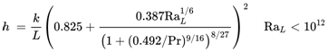
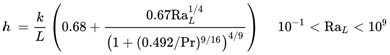
With regard to laminar flows, the following correlation is a touch more accurate. It is oberserved that a transition from a laminar to a turbulent boundary occurs when RaL exceeds around 10.
Extternal flow, vertical cylinders
For cylinders and vertical axes, the expressions for plane surfaces and be used provided so long as there isn’t a significant curvature effect. This represents the limit where boundary layer thickness is small relative to cylinder diameter D. The correlations for vertical plane walls can be used when

where GrL represents what is known as the Grashof number.
External flow, horizontal plates
Following suggestions made by W.H.McAdams a link for horizontal plates was made. The induced buoyancy can be different but to what extent depends upon whether or not the hot surface is facing up or down.
For a hot surface facing up, or a cold surface facing down, for laminar flow the following applies:
![]()
while for turbulent flow it is the following:
![]()
When the hot surface faces down, or a cold surface facing up, for laminar flow the correct formula is:
![]()
The characteristic length is the ratio of the plate surface area to perimeter. If the surface is inclined at an angle θ with the vertical then the equations for a vertical plate by Churchill and Chu may be used for θ up to 60°; if the boundary layer flow is laminar, the gravitational constant g is replaced g cosθ when calculating the Ra term.
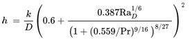
External flow, horizontal cylinder
For cylinders of sufficient length and negligible end effects, Churchill and Chu the following correlation for 10-⁵ < RaD < 10¹².
External flow, spheres
For spheres we apply the following correlation for Pr≃1 and 1 ≤ RaD ≤ 10⁵.
NuD = 2 + 0.43RaD1/4
Forced convection
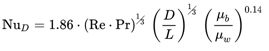
Internal flow, laminar flow
Thanks to Sieder and Tate we now use the following correlation to account for entrance effects in laminar flow in tubes where D is the internal diameter µÞ is the fluid viscosity at the bulk mean temperature µw is the viscosity at the tube wall surface temperature.
For fully developed laminar flow, the Nusselt number is constant and equal to 3.66. Mills combines the entrance effects and fully developed flow into one equation
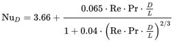
Internal flow, turbulent flow
What is known as the Dittus-Bölter correlation (1930) is a common and relatively simple correlation useful for many applications. This correlation is particularly applicable when the only viable method of heat transfer available is forced convection; i.e., there is no boiling, condensation, significant radiation, etc. Although not the most accurate correlation, its accuracy has been calculated to somewhere in the region of ±15%, it is still widely used and provides an answer within acceptable tolerances for many applications.
For a fluid flowing in a straight circular pipe that has a Reynolds number between 10,000 and 120,000 (in the turbulent pipe flow range), when the fluid’s Prandtl number is between 0.7 and 120, for a location far from the pipe entrance (more than 10 pipe diameters; more than 50 diameters according to many authors) or other flow disturbances, and when the pipe surface is hydraulically smooth, the heat transfer coefficient between the bulk of the fluid and the pipe surface can be expressed explicitly as:
![]()
where:
d is the hydraulic diameter
k is the thermal conductivity of the bulk fluid
µ is the fluid viscosity
j mass flux
cp isobaric heat capacity of the fluid
n is 0.4 for heating (wall hotter than the bulk fluid) and 0.33 for cooling (wall cooler than the bulk fluid).
The fluid properties necessary for the application of this equation are evaluated at the bulk temperature thus avoiding iteration.
Forced convection, external flow
In analysing the heat ttransfer associated with the flow past the exterior surface of a solid, the situation is complicated by phenomena such as boundary layer separation. Various authors have correlated charts and graphs for different geometries and flow conditions. For flow parallel to a plane surface, where χ is the distance from the edge and L is the height of the boundary layer, a mean Nusselt number can be calculated using the Colburn analogy.
Thom correlation
There exist simple fluid-specific correlations for heat transfer coefficient in boiling. The Thom correlation is for the flow of boiling eater (subcooled or saturated at pressures up to about 20 MPa) under conditions where the nucleate boiling contribution predominates over forced convection. This correlation is useful for rough estimation of expected temperature difference given the heat flux:
ΔTsat = 22.5 · q0.5 exp(-<em?P/8.7)
where:
ΔTsat is the wall temperature elevation above the saturation temperature, K
<em?q is the heat flux, MW/m2
P is the pressure of water, MPa
Note that this empirical correlation is specific to the units given.
Heat transfer coefficient of pipe wall
The resistance to the flow of heat will vary depending on the material of pipe, but it can be expressed as a “heat transfer coefficient of the pipe wall”. However, one needs to select if the heat flux is based on the pipe inner or the outer diameter. Selecting to base the heat flux on the pipe inner diameter, and assuming that the pipe wall thickness is small in comparison with the pipe inner diameter, then the heat transfer coefficient for the pipe wall can be calculate as if the walls were not curved:
hwall = k/χ
Where k is the effective thermal conductivity of the wall material and χ is the wall thickness.
If the above assumption does not hold, then the wall heat transfer coefficient can be calculated using the following expression:
hwall = 2k/di In(do /di)
where di and do are the inner and outer diameters of the pipe, respectively.
The thermal conductivity of the tube material usually depends on temperature; the mean thermal conductivity is often used.
Combining convective heat transfer coefficients
For two or more heat transfer processes acting in parallel, convective heat transfer coefficients simply add:
h = h1 + h2 + …
For two or more heat transfer processes connected in series, convective heat transfer coefficients add inversely:
![]()
For example, consider a pipe with a fluid flowing inside. The approximate rate of heat transfer between the bulk of the fluid inside the pipe and the pipe external surface is:
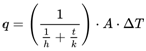
where
q = heat transfer rate (W)
h = convective heat transfer coefficient (W/m2·K))
t = wall thickness (m)
k = wall thermal conductivity (W/m·K)
A = area (m2)
ΔT = difference in temperature
Overall heat transfer coefficient
The overall heat transfer coefficient U is a measure of the overall ability of a series of conductive and convective barriers to transfer heat. It is commonly applied to the calculation of heat transfer in heat exchangers, but can be applied equally well to other problems.
For the case of a heat exchanger, U can be used to determine the total heat transfer between the two streams in the heat exchanger by the following relationship:
q = U AΔTLM
where:
q = heat transfer rate (W)
U = overall heat transfer coefficient (W/(m2·K))
A = heat transfer surface area (m2)
ΔTLM = logarithmic mean temperature difference (K).
The overall heat transfer coefficient takes into account the individual heat transfer coefficients of each stream and the resistance of the pipe material. It can be calculated as the reciprocal of the sum of a series of thermal resistances (but more complex relationships exist, for example when heat transfer takes place by different routes in parallel):
![]()
where:
R = Resistance(s) to heat flow in pipe wall (K/W)
Other parameters are as above.
The heat transfer coefficient is the heat transferred per unit area per kelvin. Thus area is included in the equation as it represents the area over which the transfer of heat takes place. The area for each flow will be different as they represent the contract area for each fluid side.
The thermal resistance due to the pipe wall is calculated by the following relationship:
![]()
where
χ = the wall thickness (m)
k = the thermal conductivity of the material (W/(m·K))
A = the total area of the heat echanger (m²)
This represents the heat transfer by conduction in the pipe.
The thermal conductivity is a characteristic of the particular material. Values of thermal conductivities for various materials are listed in the list of thermal conductivities.
As mentioned earlier in the article the convection heat transfer coefficient for each stream depends on the type of fluid, flow properties and temperature properties.
Some typical heat transfer coefficients include:
• Air – h = 1- to 1– W/(m²K).
• Water – h = 500 to 10,000 W/(m²K).
Thermal resistance due to fouling deposits:
Often during their use, especially when used on industrial portable air conditioning units with missing filters, heat exchangers can collect a layer of dirt or dust on the surface which, in addition to potentially contaminating a stream, has a detrimental effect the performance of heat exchangers. On a dirty or contaminated heat exchanger the build-up of this layer on the walls creates an additional obstacle for the heat to flow through. Because of this new layer and the subsequent additional resistance within the heat exchanger the overall heat transfer coefficient of the exchanger will be reduced. The formula below can used to ascertain the new heat transfer resistance, taking into account the additional fouling resistance:
=![]()
where
Uf = overall heat ransfer coefficient for a fouled heat exchanger, w/m2K
P = the perimeter of the heat exchanger, may be either the hot or cold side perimeter however, it must be the same perimeter on both sides of the equation, m
U = overall heat transfer coefficient for an unfouled heat exchanger, w/m2K
RfX = fouling resistance on the cold side of the heat exchanger, m2K/W
RfH – fouling resistance on the hot side of the heat exchanger, m2K/W
Pc = perimeter of the cold side of the heat exchanger, m
PH = perimeter of the hot side of the heat exchanger, m
This equation combines the overall heat transfer coefficient of an unfouled heat exchanger together with the fouling resistance and therefore calculates the total heat transfer coefficient for a fouled heat exchanger. The equation take into account that the perimeter of the heat exchanger will be different on both hot and cold sides. The perimeter used to the P does not matter as long as its is the same. The overall heat transfer coefficients will adjust to take into account that a different perimeter was used as the product UP will remain the same.
The fouling resistances can be more accurately calculated for a specific heat exchanger if the average thickness and thermal conductivity of the material fouling the coil are known. The product of the average thickness and thermal conductivity will result in the fouling resistance on a specific side of the heat exchanger.
= Rf df/kf
Where
df average thickness of the fouling in a heat exchanger, m
kf thermal conductivity of the fouling W/mK.
With almost four decades experience in the design, manufacture and supply of large portable air conditioning units, large electric fan heaters, commercial or building site dehumidifiers, infrared heaters, ventilation fans, cooling fans, fume extractor fans, portable boilers, fan coil units we’ve been around long enough to offer an unrivalled service. For details on our full range of portable climate control equipment please see our site, call 01527 830610 or drop us a line at sales@broughtoneap.co.uk where a member of the team will be only too happy to help.